Today we’ll build a model to predict a residential household energy consumption. Previous post describes the way we obtained, cleaned and pre-processed data and investigated the influence of different home attributes on it.

Model Selection

To select the best model 4 different ML models have been explored: ElasticNet, SVM, Neural Network (multilayer perceptron), and LightGBM.   Also, to select the best subset of features, models with different sets of features have been used.

Data has been split to test and trains set (85% for training and 15% for testing), and 5-fold cross-validation have been used for hyper-parameters tuning.

R2 and MSE for every model are recording for every model.

Here is an example of fitting a model (LGBMRegressor in this case):

from lightgbm import LGBMRegressor
 
parameters = {
    "boosting_type": ["gbdt"],
    "metric": ["rmse"],
    "num_leaves": [20, 50, 100],
    "bagging_fraction": [0.2, 0.4],
    "feature_fraction": [0.2, 0.4],
    "learning_rate": [0.01, 0.001],
    "lambda_l2": [2, 5],
}


model = LGBMRegressor(n_estimators = 40000)
gm_cv = GridSearchCV(model, parameters, cv=5, n_jobs=16)

gm_cv.fit(X_train, y_train)

As a preprocessing step, data has been scaled and categorical variables have been one-hot encoded.

LightGBM with abd without one-hot encoding

Although, according to LightGBM method documentation, it is common to represent categorical features with one-hot encoding, but this approach is suboptimal for tree learners. Particularly for high-cardinality categorical features, a tree built on one-hot features tends to be unbalanced and needs to grow very deep to achieve good accuracy.   That’s why I tried both approaches: to feed LightGBM one-hot encoded data and to let LightGBM deal with categorical values on its own to see if this will lead to better performance.

The first approach let to 0.71 test R2 score, while second to 0.74. So I keep using the results of the second approach as a metric for LightGBM.

Feature Engineering

For feature engineering, I used Neural Networks and SVM methods for subsets of variables (top 144, 200, 300, and 400 features).

I used two methods to select the top features: the most n important features according to the feature importance metric of LightGBM, and SelectKBest method.

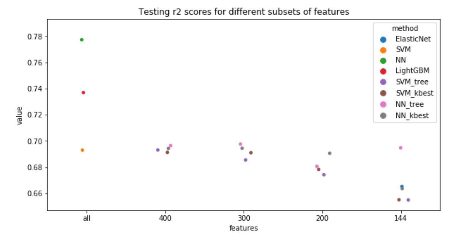
To visualize the results of all methods tried, the following plot has been generated:

According to this plot, the best performance has the neural network on a full subset of variables, with a test score of 0.78, followed by LightGBM with 0.74.

Using a subset of variables doesn’t improve the overall result. But, if we are interested in collecting fewer features to make a prediction, we can use NN with 144 features, which are suggested by LightGBM.

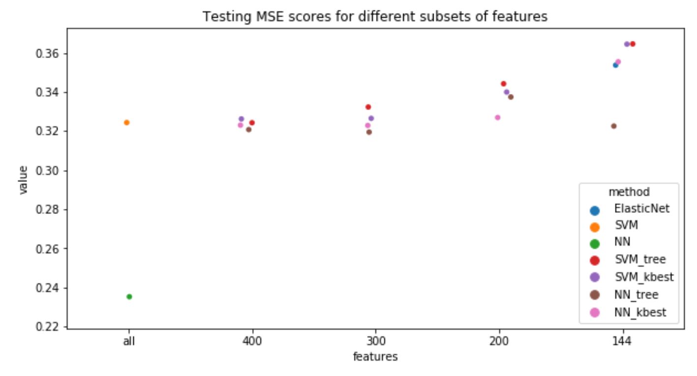
LightGMB is excluded from MSE plot, as the input data for it is not preprocessed, so it not comparable with other methods in absolute value. This plot shows the same tendency as with R2.

Although neural network gives the best performance, it’s very hard to make interpretation from it. So let’s use the next best method - LightGBM for feature interpretation.

Features importance

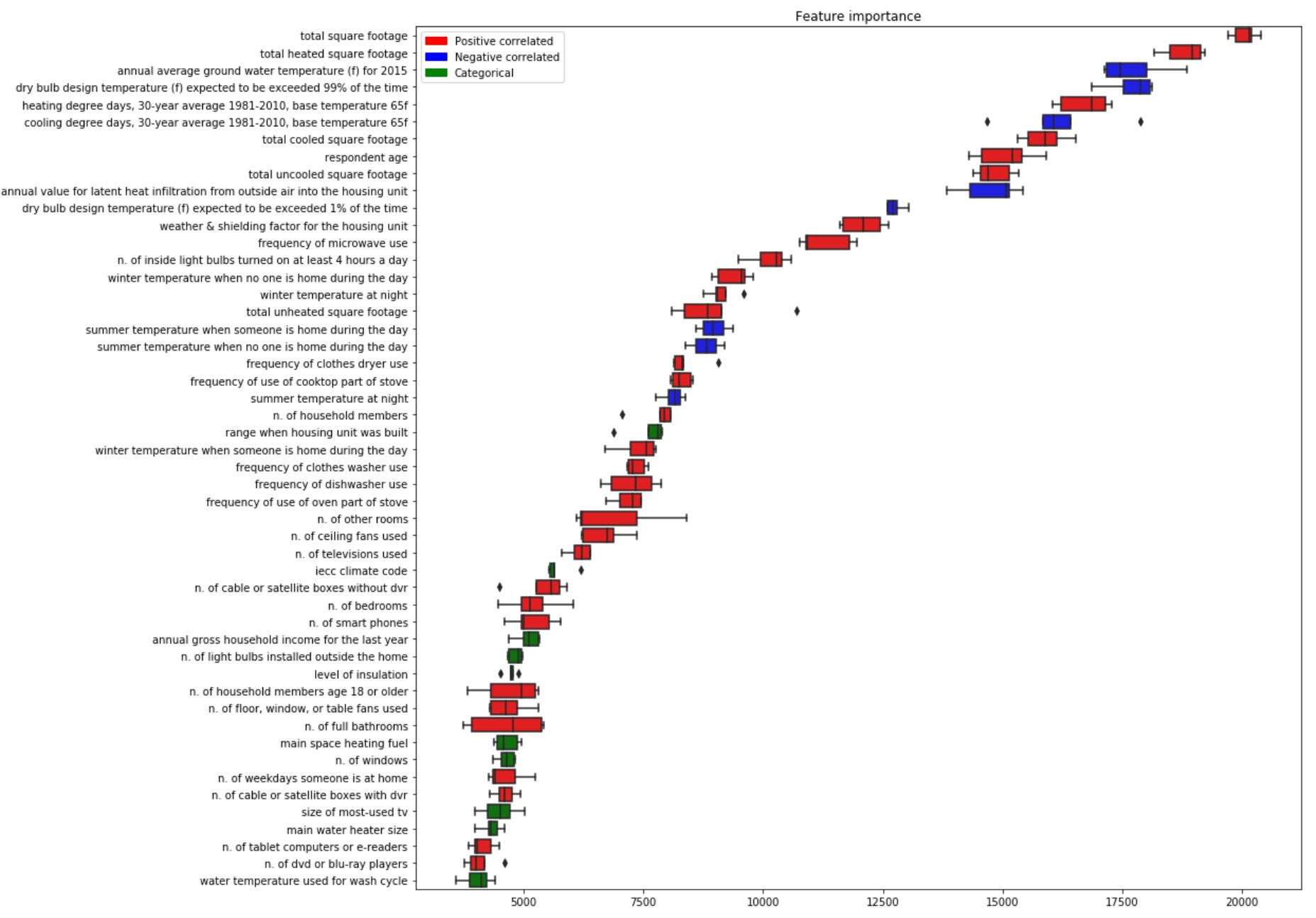
Let’s investigate the features which affect the prediction the most based on LightGBM method. To be sure that feature importance we observe is not just a property of a certain run of the model, I used the outcome from 5 models obtained from cross-validation.

Red boxplots mean that the feature is positively correlated with the outcome, blue - negative, and green - it ‘s a categorical feature.

Top 50 variables are as follows:

The spread of importance is fairly small, so we can assume that the results are stable.

Having a good predictor is good, but the real impact it’ll have only when used in real world. In our next post I’ll tell you about business application of the model we just created.